Teaching Mask R-CNN to measure something 30 pixels long
A primary cilium is about the size of a rounding error. A 1024×1024 confocal microscope image has about a million pixels; a cilium is maybe 30 pixels long and covers 20 to 60 of them. And biologists don't just want to know where it is. They want its length, and how bright each of its three parts is. Until now that meant days of drawing tiny polygons by hand in ImageJ, slice by slice.
Together with biologists from the Health and Medical University, we built CiliAI to do it in minutes. The preprint is written for biologists. This post is the developer version: what we actually did, the tricks that mattered more than the model, and one decision I would reverse.
The 30-second biology
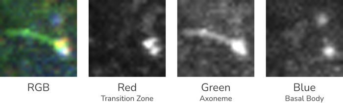
A cilium is a small antenna sticking out of a cell. For our purposes it has three parts: the basal body at the bottom, the transition zone (a short "gate" above it) and the axoneme, the long shaft. Each part is stained with a different fluorescent marker, so the image is basically RGB where every channel highlights one part: blue = basal body, red = transition zone, green = axoneme.
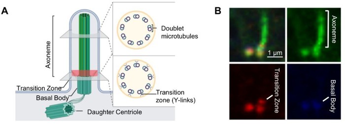
That's all the biology you need. The rest is a small-object detection and segmentation problem.
The data
The input isn't a photo. It's a 3D stack: dozens of 2D slices through the cell at different depths. 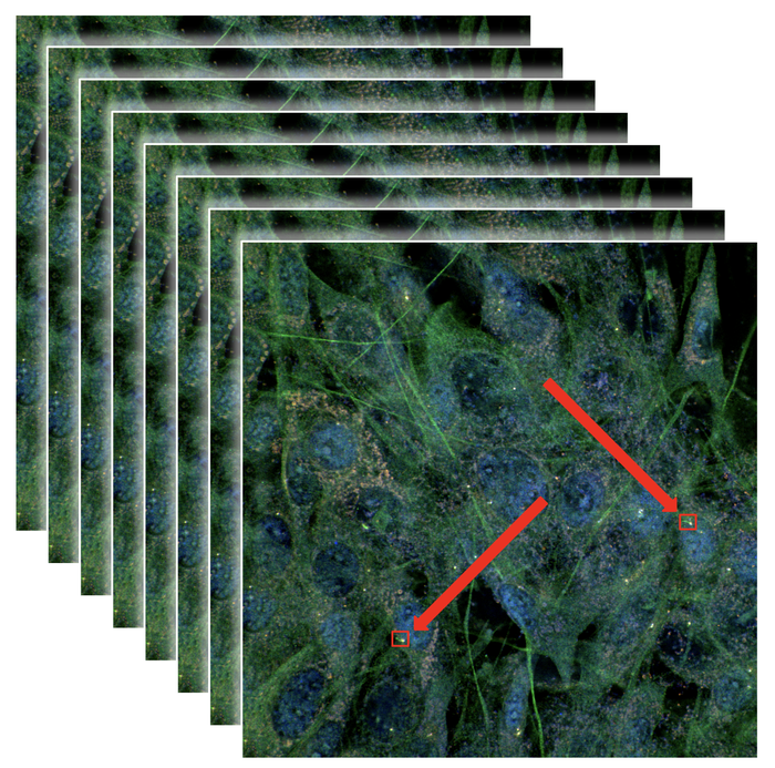
Neighbouring slices are almost identical, so we kept every fifth one. That gave about 500 unique images from just over 50 stacks.
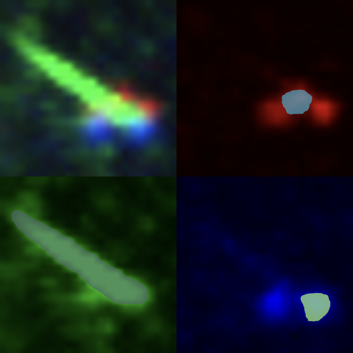
We annotated them on Datamarkin with Segment Anything doing the first pass and a human correcting it. One trick helped the annotators a lot: for every cilium we showed the RGB image next to the three channels on their own. In the merged image, a red transition zone sitting on a blue basal body is easy to misjudge. In its own channel, it's obvious.
Two models, not one
Could one model find cilia in the full image and outline their three parts? Maybe, but probably not well. The two jobs are really different: the first is finding extremely small objects in a big, busy image; the second is finding the parts inside one of those objects once it's been enlarged. At full-image scale, the parts are only a handful of pixels each.
So we split the job:
- A detection model finds cilia in the full image.
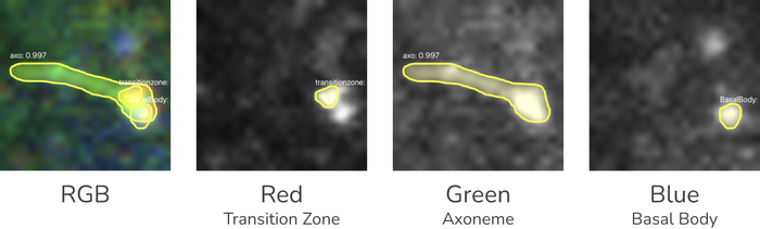
- A segmentation model gets one cropped, enlarged cilium at a time and segments its basal body, transition zone and axoneme.
Each model works at a scale where the thing it cares about is actually visible. Both are plain Mask R-CNN from Detectron2.
The small-object tricks
This is where most of the accuracy came from.
Tiling with overlap. Each 1024×1024 slice is cut into a 2×2 grid of tiles with 20% overlap (about 614 px each). The overlap means a cilium sitting on a tile border is always complete in at least one tile.
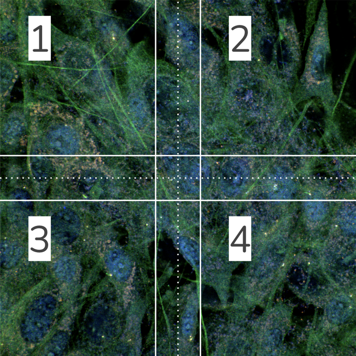
Upscaling before detection. Each tile is upscaled to 1200×1200 before going into the detector. The model doesn't get any new information, but a 30 px long cilium becomes about 60 px long, which is much closer to what the network's feature maps handle well.
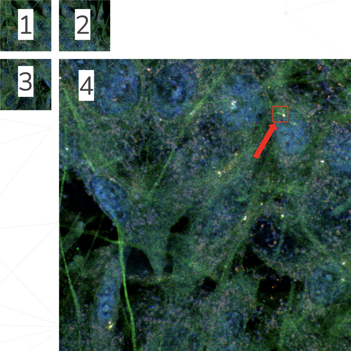
Merging duplicates. Detections are mapped back to full-image coordinates. Because tiles overlap, the same cilium can show up twice. Any two boxes with an IoU of 0.5 or more are treated as the same cilium, and we keep the one with the higher confidence. That's just non-maximum suppression across tiles.
Crop, pad, upscale for segmentation. Every detected cilium is cropped with a 10% margin, padded to a square so it isn't distorted, and resized to 1024×1024 with cubic interpolation. The second model only ever sees one big, centred cilium.
From masks to numbers
A mask isn't a result. Biologists need numbers, so the last step turns polygons into measurements:
- Length is the longest distance inside the axoneme mask, not the bounding-box diagonal. Cilia bend, and this handles that.
- Area of each part comes from its polygon (shoelace formula), converted to real units with the microscope's pixel size.
- Brightness is read from the original image data, not the upscaled crops. It's normalised by bit depth (8, 12 or 16-bit) and background-corrected. Background is simply the mean of the darkest 2% of pixels in the stack.
- Polygons are simplified with Ramer–Douglas–Peucker (1 px tolerance), which cut the stored mask data by about 70–80% with no visible loss.
- Slices are linked: a cilium found in consecutive slices with overlapping boxes is the same cilium, which tells you how deep it extends.
Reading the metrics without a PhD
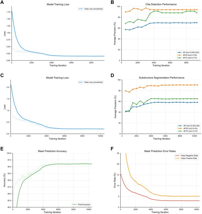
The detection model reached an AP50 of 97% but an AP of 67.5%. That looks contradictory until you know what the numbers mean:
- AP50 counts a prediction as correct if it overlaps the ground truth by at least 50%. Roughly: "did you find it?"
- AP (averaged over IoU 0.50 to 0.95) gets stricter and stricter about the exact outline. Roughly: "did you trace it perfectly?"
For objects this small, a one-pixel difference on the border is a big part of the IoU. Finding cilia is basically solved; tracing them pixel-perfectly is hard.
The segmentation model shows the same pattern per part: axoneme 74.8%, basal body 65.4%, transition zone 34.0%. The transition zone is the hardest by far: it's literally a few pixels in a million-pixel image, and its shape varies a lot. Even after cropping and upscaling, there isn't much there to learn from. It's the obvious next thing to improve.
The leak we didn't have
If I had to pick one lesson for other developers, it's this one. Our tiles overlap, and slices from the same stack look almost the same. If you split train and validation randomly by tile, near-copies of your validation images end up in training and every metric looks great for the wrong reason.
We split by source stack: no tile, crop or slice from a validation stack is ever seen in training. The numbers are lower than a random split would give, but they are honest.
Boring on purpose
Both models use Detectron2's default mask_rcnn_X_101_32x8d_FPN_3x config. No architecture changes, no hyperparameter search. Almost all the gains came from the data and the tiling, cropping and upscaling around the model. If you're working on small objects, spend your time there before touching the network.
What I would do differently: file formats
CiliAI reads Olympus .oir files, and support for Zeiss .czi and a few others was on the roadmap. In hindsight, that was a mistake.
The result today: if your file isn't .oir, CiliAI simply doesn't work for you. And getting even that one format right was a mess.
Microscope formats are proprietary, and every one has its own surprises. Reading the metadata (pixel size, slice spacing, which channel is which) is complicated. Some .czi files carry it, others need a second companion file just to be opened. Working out what each channel actually represents is its own puzzle. Even .oir wasn't clean: as far as I can tell, the camera records 10-bit data, which Python libraries don't handle well. So we read the pixel values, guess the real bit depth from them, and normalise everything to 16-bit before any of the actual work starts.
All of that took a surprising amount of development time, and none of it made the AI any better.
What I should have done: accept a simple stack of images, one PNG per z-slice (or a multi-layer image), plus three numbers for pixel size, slice spacing and channel order. Every microscope's software can export that. The format work would have been the user's one-time export instead of our ongoing maintenance.
Did it work?
On the biology side, CiliAI's length measurements matched manual measurements with no significant difference. It reproduced a known biological effect, and just as importantly, it didn't invent an effect in a condition where manual analysis found none. A model that produces false findings is worse than no model at all.
What used to take days now takes minutes.
- Preprint: CiliAI on bioRxiv
- Code, weights and training logs: github.com/datamarkin/ciliai